Section 1.1 Insights and ODEs

Subsection 1.1.1 ODEs and IVPs

We begin by reminding ourselves what, in a purely mathematical sense, a differential equation is.

Definition 1.1.1. First-Order Ordinary Differential Equations.

Let \(t\) denote time, which we will take as our independent variable throughout this text. A first-order ordinary differential equation (ODE) is an equation involving some unknown function of \(t\text{,}\) \(y\) (the dependent variable), its derivative \(y'\text{,}\) and possibly \(t\text{.}\) If possible, we often write our first-order differential equations in the standard form
\begin{equation*} y' = f(t,y), \end{equation*}
where \(f\) is some function of \(y\) and \(t\text{.}\) A solution to an ODE is some representation (not necessarily as a formula!) of a function that makes the equation true when substituted for \(y\text{.}\)
An initial value problem (IVP) is an ODE together with some specified output value at a specified input value, expressed as \(y(t_0) = y_0\text{,}\) i.e. we are told that the graph of the unknown function \(y\) passes through the point \((t_0,y_0)\text{.}\) The equation \(y(t_0) = y_0\) is called an initial condition and the value \(y_0\) is the initial value.
In more practical terms, a first-order ODE informs us of how this unknown function relates to its own derivative (rate of change) and time. The practical value of this idea is that we can often express or measure how a quantity changes more easily than find an expression for its value. Each ODE will have an entire parametrized family of functions as its set of solutions and the initial conditions indicate a data point in the \(ty\)-plane that the graph must pass through. This picks out a particular solution. We will see later that we may have many data points and parameters in the ODE which we can (approximately) solve for using optimization.
Here are three examples that may help make the idea of ODEs and IVPs make sense. We will develop these as Insights before the end of the section.

Example 1.1.2. Linear Functions.

The first initial value problem you probably ever encountered was most likely stated in the following form: find the equation of a line with slope \(m\) passing through the point \((t_0,y_0)\). Stated in terms of differential equations, this instruction is simply to solve the IVP
\begin{equation*} y' = m, y(t_0) = y_0. \end{equation*}
The solution (check it), in slope-intercept form, is
\begin{equation*} y = mt + (y_0 - mt_0). \end{equation*}
Observe that in practical situations, \(y\) and \(t\) typically have some sort of units. The units of \(y'\text{,}\) and thus \(m\text{,}\) are \(\frac{y\text{ units}}{t\text{ units}}\text{.}\)

Example 1.1.3. Exponential (Malthusian) Growth.

The second common family of functions that naturally arises as the set of solutions to a family of differential equations are exponential functions. Here we will let our dependent variable be \(P\) (for population, measured in individuals) and out independent variable be time, \(t\text{,}\) in whatever units make sense for the problem.
The defining feature of a population that is growing exponentially is the following: the instantaneous growth rate in \(P\) is proportional to \(P\text{,}\) with some constant of proportionality \(k\). Assuming \(P(t_0) = P_0\text{,}\) finding the population as a function of time amounts to solving the IVP
\begin{equation*} P' = kP, P(t_0) = P_0. \end{equation*}
The solution to this IVP is given by \(P(t) = P_0e^{kt}\)
Observe that the units of \(P'\) are \(\frac{\text{individuals}}{\text{time}}\text{.}\) Since \(P\) has units of individuals, in order for the differential equation to be dimensinally consistent the units of \(k\) must be \(\frac{1}{\text{time}}\text{.}\) This is a commonly encountered unit for percent rates of change because percentages are by definition dimensionless.

Example 1.1.4. A System of IVPs.

Now we will introduce the idea of a system of differential equations. A system of ODEs (hence IVPs) involves multiple dependent variables whose rate of change depend on one-another. Such situations arise all the time. For instance, the variables could be competing animal species, interacting sub-populations during an epidemic (those who are susceptible, infected, and recovered), or the position and velocity of a mass on a spring.
A particularly simple example is given by
\begin{align*} x' = -y,\amp\ \ x(0) = 1\\ y' = x,\amp\ \ y(0) = 0. \end{align*}
In this example we are using \(x\) and \(y\) as the dependent variables to describe the coordinates of a particle moving in the \(xy\)-plane. The values of \(x\) and \(y\) describe the particle’s position, whereas the values of \(x'\) and \(y'\) decribe where it is moving (instantaneously). More specifically, let’s think about the motion of the particle decriped by the differential equations when it is in each of the four quadrants of the plane.
  • If \((x,y)\) is in the first quadrant, \(x\) and \(y\) are both positive. Looking at the equations, we see that this means \(x'\) is negative and \(y'\) is positive. Thus, the particle is moving up and to the left.
  • If \((x,y)\) is in the second quadrant, \(x\) is negative and \(y\) is positive. Looking at the equations, we see that this means \(x'\) is negative and \(y'\) is also negative. Thus, the particle is moving down and to the left.
  • If \((x,y)\) is in the third quadrant, \(x\) and \(y\) are both negative. Looking at the equations, we see that this means \(x'\) is positive and \(y'\) is negative. Thus, the particle is moving down and to the right.
  • Finally, if \((x,y)\) is in the fourth quadrant, \(x\) is positive and \(y\) is negative. Looking at the equations, we see that this means \(x'\) is positive and \(y'\) positive. Thus, the particle is moving up and to the right.
The motion described above sounds like it might be circular (or at least periodic). Indeed, the solution to the given system of IVPs is \(x(t) = \cos(t)\) and \(y(t) = \sin(t)\text{.}\) As \(t\) changes, the particle traces out the unit circle. Varying the initial conditions will change the starting point, which will change the radius if the starting point is not one unit from the origin.
Subsection 1.1.2 Insights of IVPs

Now let’s get to the heart of this text: Insightmaker and Insights. If you haven’t already, you’ll want to go to Insightmaker.com and create a free account. Also, if you were reading the three examples in the previous subsection and weren’t feeling extra enlightened, the goal of this section is to help us see what’s going on by visualizing ODEs in multiple ways.

Definition 1.1.5. Insight.

Insightmaker represents ODE (systems-dynamics) models (on pages called Insights) using what are known as stock-flow models. Here we list the basic components of a stock-flow model, called primitives. Each component will be discussed in more depth separately.
  • Stocks: Stocks are things that accumulate. In the context of modeling with ODEs, these are the dependent variables of the system.
  • Flows: Flows into a stock contribute positively to the time-derivative of the corresponding dependent variable. Likewise, outflows contribute negatively. Briefly, the key formula to manage a stock-flow model is the following:
    \begin{equation*} \mbox{Time Derivative of a Stock} = \sum\mbox{Inflows} - \sum\mbox{Outflows} \end{equation*}
  • Variables: Variables are often used as parameters in the context of ODEs. These are numbers that we may modify to match our model to data, such as adjusting \(k\) in Example 1.1.3 in order to match a value of the population at a later time.
  • Links: Links are arrows between stocks, flows, and variables that allow the linked objects to be used in the formulas for the object that the to which the link points. Yes, that’s a mouthful, but links are quite a useful organizational tool.
Now we can take each primitive individually and say
  1. How it is created.
  2. How it can be modified.
  3. What its important settings are.
Following along through each primitive, you can create an Insight for Example 1.1.2.

Primitive Summary 1.1.6. Stocks.

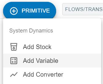
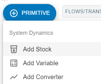
  1. To create a stock, click on the "\(\oplus\) PRIMITIVE" button and choose to add a stock as shown. This will create a blue rectangular box with the name of your stock, which you can edit on the right side of the Insightmaker screen. Call this one \(y\text{.}\)
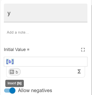
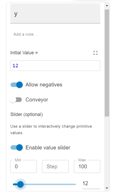
  2. When the stock you have created is highlighted, you will see this box on the left side of the Insightmaker screen. This is where you can set the initial value of the stock. This will be the value of the stock at the start of the simulation (the default start is at \(t = 0\)). Here we have it set to the value \(12\text{.}\) Perhaps the most important mathematical idea with stocks is the following: The expression you enter for the initial value is a single number, not something that varies with time; the time evolution of a stock is determined by the flows, which can depend on time.
    When we discuss variables and links, we will let the initial value be a variable. Doing this makes sense in models where we think of the initial value as a parameter, such as \(b\) in \(y = mx+b\text{.}\)
  3. Now we will discuss the only two settings we use for stocks in an introductory Differential Equations course.
    • We will typically want "Allow negatives" to be on, i.e. the stock can take on negative values. Even in models where context might exclude negative values (such as when a stock is population), we would like to allow them anyway so that we can see something might be wrong with our model.
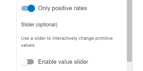
    • If you toggle on "Enable value slider", this will allow you to create a slider for the initial value of the stock. The ability to use sliders in simulations and see how the behavior of the model changes dynamically is one of the most useful features of Insightmaker. (In the Insight we’re building, we will disable the value slider for this stock and create a variable for \(b\) with a slider enabled.)

Primitive Summary 1.1.7. Variables.

  1. To create a variable, click on the "\(\oplus\) PRIMITIVE" button and choose to add a variable as shown. This will create a peach-colored ellipse with the name of your variable, which you can edit on the right side of the Insightmaker screen. Create two variables called \(m\) and \(b\) (drag so they’re not on top of one another).
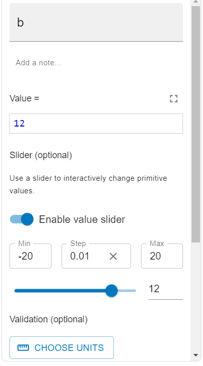
  2. Similar to stocks, when a variable you have created is highlighted, you will see this box on the left side of the Insightmaker screen. This is where you can set the value of the variable. This will be the value of the variable through at the start of the simulation. Note that there is a lot of flexibility in what we may enter in the formula for a variable; it may be a function of time or depend on other variables. In the example we’re exploring our variables will be the slope and \(y\)-intercept of a linear function, which will be numbers controlled by sliders.
    Links (discussed below) will allow our new variables to be used in formulas for other primitives.
  3. The main setting we use for variables allows them to be dynamic parameters in simulations.
    • If you toggle on "Enable value slider", this will allow you to create a slider for the numerical value for the variable. When the slider is enabled and a numerical value is chosen, that variable will be constant through the simulation. You can choose a range of values and a step size for the slider that you find useful. Here we chose a range of \(-20\leq b\leq 20\) with a step size of \(0.01\) and set the slider to \(12\text{.}\)

Primitive Summary 1.1.9. Flows.

  1. To create a flow, click on the "Flows/Transitions" button to highlight it. Now click on the stock which you want to be the source or target of your flow (if the flow really has no source, click on the target stock only). Then you can drag the arrow to the stock at the other end of the flow. If there is no stock at one end, you will have a cloud at one end of the flow. In our example we want a flow with a cloud as source and \(y\) as its target.
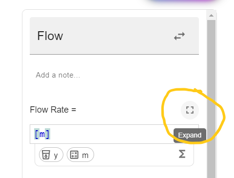
  2. When the flow is highlighted you will see this box on the left side of your screen. You may modify the formula for the flow in the current window, or you can click the circled box to have a new formula editing window. The formula may involve time (entered as Seconds(), Minutes(), etc.), the upstream and/or downstream stocks, or any linked variables. In our example we should link \(m\) to the flow into \(y\) and make it the flow rate.
    • For flows we can choose to only allow positive flow rates by toggling "positive flow rates only" on. When this is on there will be no flow from the target to the source. This will make sense to do in some contexts but not others. In our running example, if we wish to allow for negative slopes, then we need to toggle this feature off.
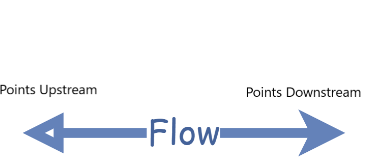
    • When negative flow rates are allowed, we need to know which direction of the flow arrow positive rates represent. This is observed by one end of the the bidirectional flow arrow being hollow. Positive flow rates go from the primitive at hollow arrowhead to the primitive at the filled arrowhead.
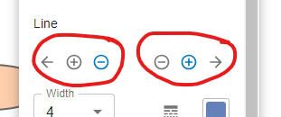
      Additionally, you may assign a minus sign (\(-\)) and a plus sign (\(+\)) to the ends of the arrows indicating positive and negative flow directions as this is somewhat easier to see than the default arrowhead types. To do this, right click on the flow and scroll down to see the "line" options and choose a minus on the start arrow and plus on the end arrow, as shown. You may choose this as the default for your insight by choosing to set this as the flow theme in the same menu.
If you have followed along building a linear function Insight as you have been reading, you should have an Insight like the following:
Figure 1.1.10. An Insight for a linear function (click on "full screen Insight" to open in a new window).
Now you can click "simulate" and we see the time evolution of \(y\) with initial value \(b\) and slope \(m\) (you may need to use the configuration settings in the simulation window to only show \(y\)). If "sliders linked" is highlighted in the simulation window, then you can dynamically change the parameter values and see the effect on the graph of \(y\text{.}\)
described in detail following the image
Linked sliders button in simulation window.

Remark 1.1.11.

Note that when sliders are linked, you may want to configure your graphing window with a fixed minumum and maximum for the axes. Otherwise, the axes will change as the parameters are varied.