
Section 3.3 Disease Models

Subsection 3.3.1 The Basic SIR Model

The basic model for the spread of an infectious disease involves three sub-populations of a larger one.
  • The sub-population of individuals who are susceptible to infection. The number of individuals in this population is denoted by \(S\text{.}\)
  • The sub-population of individuals who are infected. The number of individuals in this population is denoted by \(I\text{.}\)
  • The sub-population of individuals who are recovered from the disease. The number of individuals in this population is denoted by \(R\text{.}\)
In order to simplify the model, we assume that
  1. The total population remains constant, i.e. nobody enters or leaves the local population in which we are modeling spread of the disease.
  2. Once recovered, individuals gain immunity from re-infection. This is often true for common diseases, at least on the time scale in which we might model.
A good test-study for this situation is the case presented in [15] and develobed as a SIMIODE modeling scenario in [11]. In this scenario we have a British boarding school where an influenza outbreak occured. The number of infected students each day of the outbreak is given by the table:
Table 3.3.1. Influenza Outbreak Model
Day 0 1 2 3 4 5 6 7 8 9 10 11 12 13
\(\#\)infected 1 3 25 72 222 282 265 233 189 123 70 25 11 4
The total number of boys at the school was 763.
To build the model, we start with the rumor spread model Example 1.3.4, thinking of the infection as a rumor. Thus, we have two stocks \(S\) and \(I\text{,}\) with a flow from \(S\) to \(I\) given by the formula \(aSI\text{,}\) where \(S\) and \(I\) are in units of individuals and \(a\) is in units of \(\frac{1}{\text{individuals}\cdot\text{days}}\text{.}\) We assume that a consant percentage of the infected individuals recover on a daily basis. Hence the flow rate from \(I\) to \(R\) is given by \(kI\text{,}\) where \(k\) has units of \(\frac{1}{\text{days}}\text{.}\) This yields the Insight Boarding School Insight, with main diagram
Figure 3.3.2. The SIR model diagram.
and system of differential equations given by
\begin{align*} S' =\amp -aSI\\ I' =\amp aSI - kI \\ R' =\amp kI. \end{align*}
Initial values are given by \(S(0) = 762\text{,}\) \(I(0) = 1\text{,}\) and \(S(0) = 0\text{.}\)
To estimate \(a\) and \(k\text{,}\) we use the data given in Table 3.3.1 as a converter and use the optimization algorithm to minimize the sum of squared errors as in Boarding School Insight with Data to obtain \(a\approx 0.002\) and \(k\approx 0.5\text{.}\) This yields the time series graphs (with the data shown)
Figure 3.3.3. SIR from boarding school matched to data.
To show the total population being conserved, we can apply the "use areas" in the graph to obtain the following:
Figure 3.3.4. Using area graphs to show the conserved population in the basic SIR model.
This graphical representation is particularly nice when a sum of quantities is conserved through time. This could be total population or total energy (potential plus kinetic) in a mechanical system.

Subsection 3.3.2 Variations on the SIR Model

There are many variations on the SIR model. These variations could be mathematical or contextual in nature. A nice survey is available at [9]. A fun (or horrifying variation) is to make the infected populations zombies, as in [4]. The following exercise explores one possible variation given in Part II of [5].

Checkpoint 3.3.5.

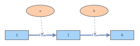
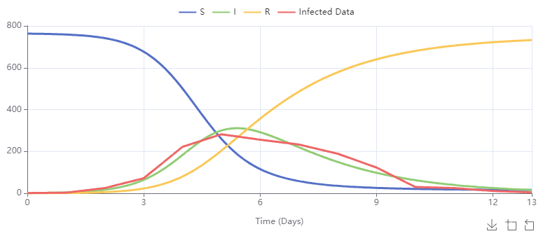
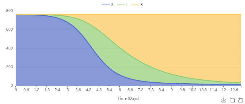
Consider the scenario where instead of "recovered", we call the stock described by \(R\) "removed" in the sense that they are removed from the \(S\) and \(I\) populations. Suppose that we have a population of \(1000\) individuals, \(I(0) = 2\text{,}\) \(S(0) = 988\text{,}\) and \(R(0) = 10\text{.}\) Let \(a=0.002\) and \(k = 0.5\text{.}\)
Now, assume further that individuals in the removed population can convince individuals in the susceptible population to practice better hygiene to avoid infection. Essentially, susceptible individuals can be "infected" with better health practices. Create a new model with a new variable \(m\) that describes this interaction in a way similar to the \(S\)-\(I\) interaction.
  1. How large does \(m\) need to be to ensure the infected population never goes above \(25\%\) of the population?
  2. What are real-world things that would impact the size of \(m\text{?}\)