A standard first-order ODE is associated to the following problem type:
Problem3.2.1.The Basic Salt Tank Problem.
A brine (salt water) solution of conentration \(C\) kg/L at a rate of \(r\) L/min flows into a tank of volume \(V\) of initially pure water. A well-mixed solution drains out the bottom of the tank at \(r\) L/min. How much salt is in the tank as a function of time?
In this section we explore this type of problem in general with multiple tanks and perhaps without conserved volumes. The worksheet in the next section presents the modeling scenario in [13] and section 6.5.1 of [3]
To present the problem in Problem 3.2.1 in ODE form, letting \(A\) denote the amount of salt in the tank at a time of \(t\) minutes, we have
\begin{equation*}
A' = rC - \frac{A}{V}r,\ A(0) = 0.
\end{equation*}
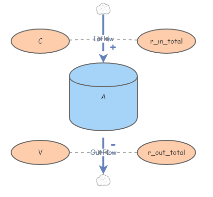
We can arrive at essentially through unit analysis. Since the amount of salt in a tank sounds exactly like a stock, we can represent it as the following Insight:
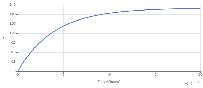
The long run equilibrium amount of salt in the tank is \(2\)kg. This makes sense as it yields a concentration of \(0.25\)kg/L. In the log run all the mixture in the tank is inflow mixture.
In your own copy of Figure 3.2.2, create a variable that is equal to \(|\text{Inflow} - \text{Outflow}|\text{.}\) For a given \(r\text{,}\)\(V\text{,}\) and \(C\text{,}\) use the optimization algorithm to find the equilibrium value of \(A\) by imnimizing the integral of this new variable.
Subsection3.2.2Two Tanks with Constant Fluid Volume
Consider the first problem:
The Two Tank Mixing Problem.
Consider two interconnected tanks initially containing fresh water, call them Tank 1 and Tank 2, of volumes \(V_1\)L and \(V_2\)L, respectively. A brine solution of concentration \(C\)kg/L flows into Tank 1 from an external source at a rate of \(r_{\text{in}}\)L/min. A well-mixed solution froms from Tank 1 to Tank 2 at a rate of \(r_{12}\) L/min and from Tank 2 to Tank 1 at a rate of \(r_{21}\)L/min. Finally, a well-mixed solution exits Tank 2 at a rate of \(r_{\text{out}}\)L/min.
Create variables for \(C\text{,}\)\(V_1\text{,}\)\(V_2\text{,}\)\(r_{\text{in}}\text{,}\)\(r_{\text{out}}\text{,}\)\(r_{12}\text{,}\) and \(r_{21}\text{.}\)
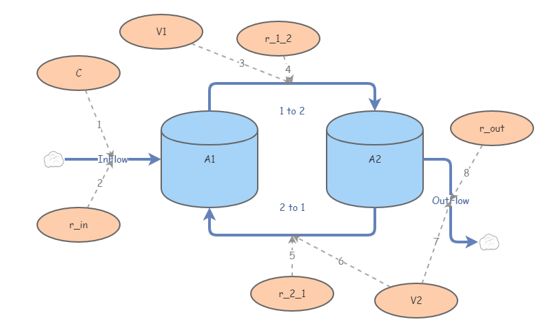
Now we need to create links based on what the various salt rates depend on. The best strategy for this is to take each tank and apply the idiom diagram shown below, which corresponds to the ODE
\begin{equation*}
A' = Cr_{\text{in total}} - r_{\text{out total}}\frac{A}{V}
\end{equation*}
While this diagram may seem complicated, we now see that each ODE in our system will have three terms, what their signs are, and on what variables they depend. We have
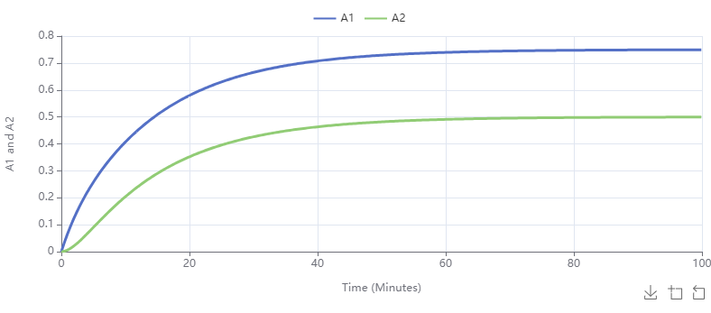
Using these to build our flow rates in the diagram. Using parameter values indicated in the table nad running for \(100\) minutes, we obtain the following (Insight):
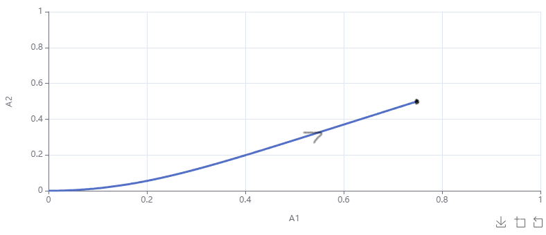
In each of these graphs we see the long run behavior yields a concentration of about \(0.25\)kg/L, as expected. We can also see the equilibrium solutions approached in the following scatter plot:
Figure3.2.9.Scatter plot for the two tank problem. Dot at the equilibrium and arrow added.
In order to allow for the volume in each tank to be variable, we create links to the volume variables, \(V_1\) and \(V_2\text{,}\) from the appropriate rate variables. Now, after removing the sliders for \(V_1\) and \(V_2\text{,}\) we may enter
in the formulas for \(V_1\) and \(V_2\text{,}\) respectively (with initial volumes as in the previous section). Note that care with units must be taken when entering these formulas; the first would be entered as {3 Liters}+([r_in]-[r_1_2]+[r_2_1])*{Minutes() Minutes}.
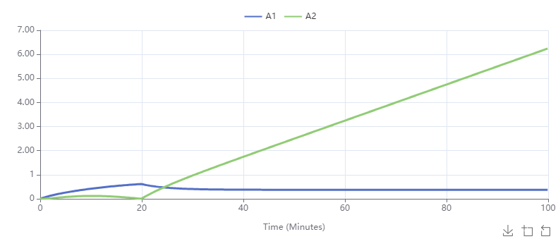
We have a problem because the volume of liquid in Tank 2 approaces zero in \(20\) minutes. This is when we can use one of the most powerful features of Insightmaker.
Using the If Then Else function in the General Functions Menu, we can add conditions to our flow rates. The syntax is given by IfThenElse(Test Condition, Value if True, Value if False).
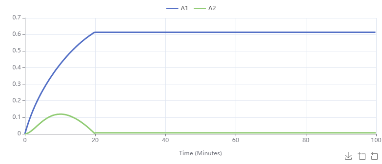
In our case we must link \(V_1\) and \(V_2\) to all flows and apply the condition that both volumes are positive to all the flow rates. For instance, the Outflow flow rate will be given by IfThenElse([V1]>{0 Liters} and [V2]>{0 Liters},[r_out]*[A2]/[V2],0). Applying this we obtain the following time series:
Figure3.2.11.Variable volume salt tank amounts using a conditional to deal with zero or negative volumes.
The Insight for this scenario may be found at Variable Volume Mixing Insight. One could argue the number of links starts to make the Insight inelegant. At this stage it might be useful to experiment with ghosting primitives (see ghosting). A slightly more visually pleasing Insight is available at with ghosts.
Try to re-create the results of the variable volume tanks using stocks for each volume. This will avoid putting explicit formulas for the volumes as functions of time.