In this section we will follow the example given in the first section [3] and [2] to show the full workflow of modeling a real-world scenario with Insightmaker. You are encouraged to build your own Insights as you work through this section. However, if you get stuck, links to three Insights are provided at the end of this section. Each one illustrates a different approach to parameter estimation.
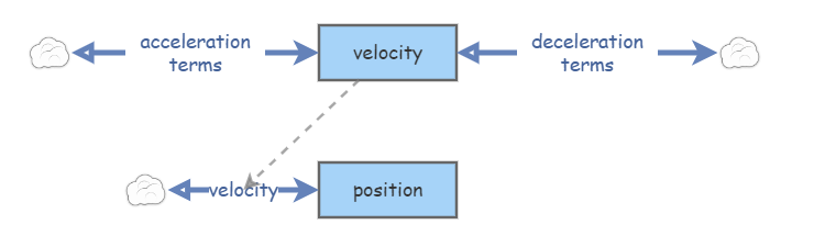
Observe that the data we are presented with is position, while we are attemting to model velocity. This turns out to be a common situation as velocity is easier to model with a differential equation using Newton’s Second Law (\(F = ma\) has the derivative of velocity on the right-hand side), whereas position is easier to measure for data collection. However, since we can numerically integrate using Insightmaker we just need to create a model for velocity, then make the velocity stock equal to the inflow rate of the position stock via a link. This idea is illustrated with the following basic diagram, which we may refer to as an idiom since it describes a very common modeling situation (this is the velocity-to-position idiom).
Creating this basic diagram for the modeling scenario, while it may seem intuitive, is the first step in the process of modeling using Insightmaker. We will now carry out the rest of the modeling process explicitly.
Modeling Step2.1.3.Step 1: Identify Stocks and Flow Relationships.
Identify all time-dependent variables (stocks) in the scenario and observe possible inflows, outflow, and flows between stocks. Decide if any stock influences the flow into or out of another and create links accordingly.
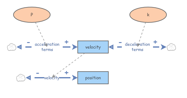
It is also good practice to establish units on all the stocks and flows of the model at this stage. In this case we will establish meters as the units of position, m/s as the units of velocity (the stock and the flow into position) and m/s\(^2\) as the units of both flows into velocity.
For the model of a sprint we will follow the Hill-Keller model as in [2]. In this model we have one term for propulsive force, \(F_p\text{,}\) which is assumed to be proportional to the mass of the sprinter. Thus,
\begin{equation*}
F_p = mP.
\end{equation*}
Here \(F\) will be in units of m/s\(^2\) and \(m\) will be in units of kilograms. We will see that only one of them (\(F\)) must be added as a variable in the model.
There is also a resistive force, \(F_r\text{,}\) that is assumed to be proportional to the velocity and the mass of the sprinter. This assumption is based on the idea that this resistive force accounts for air resistance and internal resistance of the runner’s body. Thus,
\begin{equation*}
F_r = -kmv.
\end{equation*}
Here \(k\) has units of \(1/\)s. We will add \(k\) as a variable to our insight.
\(0.005\text{.}\) This is a very small time step, but it is (sort of) necessary because of the initial point and wanting \(9.69\) to be an exact time step. (We could use a larger time step by investigating factors of \(9525\text{.}\))
At this point we have the Insight. Following [3], we will let \(P = 11\) and make \(k\) have a slider to adjust it in small steps (of size \(.001\)) between \(0\) and \(1\) (arrived at by running the model to see what works).
Modeling Step2.1.8.Step 3: Adjust Parameters to Match the Data.
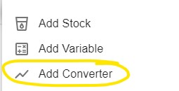
After creating some quantifiable way of measuring how well the simulation matches the data, import the data as a converter and use an optimization procedure to make the simulation match the data as well as possible.
use the built-in optimization algorithm in Insightmaker to minimize the sum of squared errors between the collection of data points and the simulation.
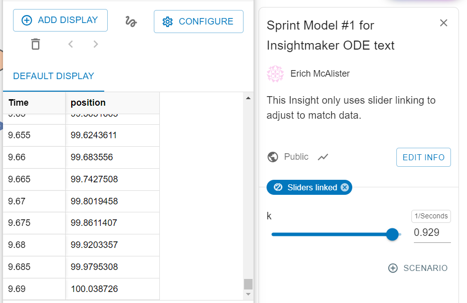
Adjust Paramteters with Sliders: This is the most intuitive method. In this case, Bolt ran \(100\) meters in \(9.69\) seconds. Thus, we can run the simulation set to display time and position in the table display. Then, with sliders linked, we can adjust \(k\) to make the position as close as we can to \(100\) as possible when \(t=9.69\text{.}\) The result is shown below:
Use the Optimizer (Version 1): As an alternative to using a slider, we can use the built in optimization algorithm to minimize \(|\text{position}-100|\) when \(t=9.69\text{.}\) First, we create a variable for \(|\text{position}-100|\) (it will need a link from position). Then we proceed as follows:
Choose "Optimization and Goal Seeking" from the "Tools" (toolbox next to the "Simulate" button).
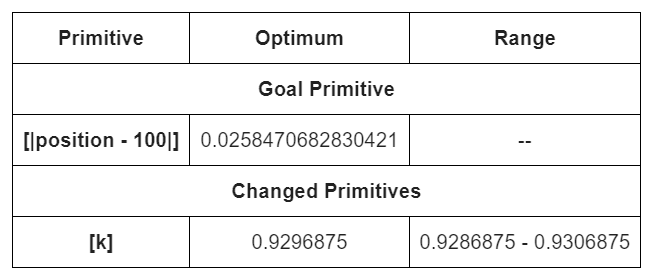
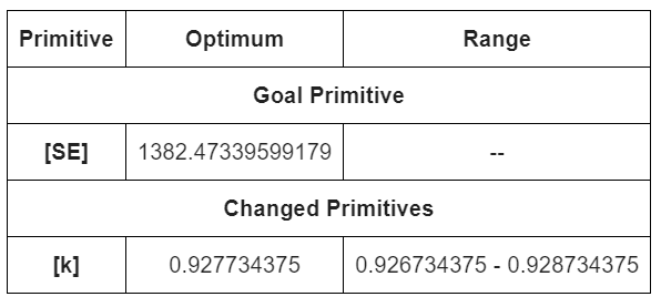
Choose \(|\text{position}-100|\) as the primitive and accuracy of \(0.001\) along with a guess range for \(k\) (determined by using sliders an visual inspection).
Running the optimization, we find the \(k\) is about what we found using the slider method. Notice we get a range of values and the value of the minimized variable. This is a numerical optimization algorithm, hence may not arrive at exact values even if you can find them by hand. The output is shown below.
Use the Optimizer (Version 2): Minimizing the difference between \(100\) and the model’s predictied position at \(t=9.69\) does not account for any other time-position pairs. To obtain a more global fit to the data, we will use a converter with the entire dataset. Then we will minimize the sum of squared errors from the data to the model outputs.
From here, insert the time and position values from Table 2.1.1 with time as input source, meters as units, and linear interpolation. (Linear interpolation builds additional data points for comparison to the simulation by drawing straight lines through the data points.)
Now open the optimization menu and choose to adjust \(k\) to minimize the integral of \(SE\text{.}\) (The integral will be the sum of the squared errors.)
Create a new stock whose flow rate is \(SE/\text{TimeStep()}\) (dividing by \(\text{TimeStep()}\) will make this into a sum rather than an integral, which is what the optimizer does, really). Use this to compare the \(SSE\) (sum of squared errors) for \(k=0.929\) and \(k=0.9277\) to verify that the latter gives a better global fit to the data.